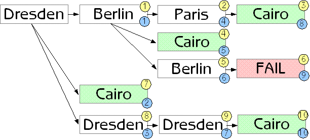
If you think about the algorithm needed to solve this problem, you will soon realize that it is really a graph search problem with the twist that the cost of moving between the nodes (cities) changes over time.
One thing that I hadn't even thought about when designing this contest was the two fundimental ways of approaching the problem of searching the graph: depth-first and breadth-first searching.
My test implementation uses depth-first searching but, after looking at some other people's solutions, it is clear that breadth-first searching offers several performance advantages. Depth-first searching, on the other hand, has the advantage of being someone easier to understand, at least by people who don't run in terror when they see recursion. Let's look at an example...
| Day 1 | Day 2 | Day 3 | ||
|---|---|---|---|---|
|
{('Dresden', 'Berlin') : $, ('Dresden', 'Cairo') : $} |
{('Berlin', 'Paris') : $, ('Berlin', 'Cairo') : $} |
{('Paris', 'Cairo') : $, ('Dresden', 'Cairo') : $} |
Above is an example schedule showing several possible routes from Dresden to Cairo (remember that you can wait in a city for as long as you want). The prices aren't relevant to the example, so they are all represented by a dollar-sign.
Below is a diagram showing all the possible routes that have to be considered to decide which is the cheapest. The numbered circles indicate the order in which these routes are evaluated. The yellow circles show the order for depth-first searching, the blue circles show the order for breadth-first searching.

As you can see from this example, it is more likely that a breadth-first search strategy will find a solution earlier in the search process. And, assuming the flight costs are random, this solution is likely to be a good solution (because taking more flights is likely to cost more than taking fewer). By finding solutions earlier, an optimized breadth-first algorithm can discard a lot of more-expensive solutions earlier, leading to a significant performance improvement.